Batch-to-Streaming Energy Forecasting with Spark ML and Kafka

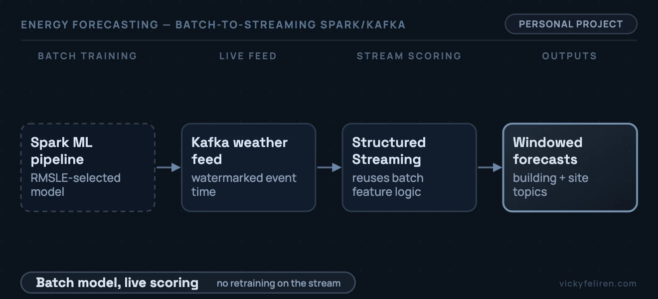
I wanted to take a model beyond a training notebook. Therefore, I used hourly meter readings, building data, and weather from several sites to predict 6-hour energy use. The saved model then scores weather events as they arrive through a live stream.

Batch training and streaming create different problems. Energy use spans about 8 orders of magnitude, from nearly empty buildings to whole campuses. Moreover, inputs mix numbers, circular wind direction, and large categories. The metric must balance absolute and relative error. Meanwhile, streamed events arrive out of order, and window state needs a memory limit. The offline model must also score events fast enough for live use.

I defined Spark schemas for all 3 tables to avoid slow schema inference. Then I chose features based on data analysis. Log1p, which applies a logarithm after adding 1, scaled floor area. Building age replaced construction year. Moreover, sine and cosine encoded wind direction so 359° stayed close to 1°. Each site’s 3 hottest and coldest months defined peak seasons.

I removed building and site IDs to prevent the trees from memorising identities. This encouraged patterns that transfer to unseen buildings.

I trained Random Forest and GBT on the same features to isolate the model choice. I selected models using RMSLE, which measures error on a logarithmic scale. Thus, a 10% error carries similar weight across small and large buildings. Random Forest beat GBT at 1.97 versus 2.29 RMSLE. Tuning then reduced it to 1.95. Training on log1p energy produced the best score, 1.30, by reducing the target’s skew.

I saved that final pipeline for streaming.

A Kafka producer replays weather records in time order. Spark Structured Streaming uses a 5-second watermark to allow expected delays while limiting stored state. Then it repeats the training features and scores each event with the saved model. Separate Kafka topics receive results from 2 tumbling windows, which group events into fixed, non-overlapping intervals. The 7-second window produces 6-hour building totals, while the 1-second window produces daily site totals. Each window matches how quickly its group gains enough useful events.

A consumer notebook reads the output topics and joins predictions with actual meter readings. Then it builds plots for operators. A heatmap across buildings and intervals flags candidates for demand response. Per-site daily trends show where consumption is heading. Moreover, a shortfall/excess chart identifies sites where predictions fall below or exceed actual use. Under-predicted sites are the urgent operational failure.

A predicted-versus-actual trace marks the largest error and traces it to a concrete cause. However, the features cannot capture isolated building events such as equipment faults or unscheduled occupancy changes. Therefore, the model smooths over these events.

I built this to test the full path from training to a realistic deployment. Therefore, training decisions had to support the later stream. The streaming job also needed to limit stored state and handle event times correctly. Moreover, it had to reuse the saved model.

Batch decisions shaped the stream more than I expected. Removing raw building and site IDs prevented leakage and let the saved model score unseen buildings. Moreover, watermarks and windows had to match both producer and consumer clocks. Therefore, I needed to tune both sides together.

Before deployment, I would add Kafka access controls because short-interval building forecasts can reveal identity or occupancy. The largest errors come from faults and occupancy changes absent from the features. Therefore, the next model needs these signals. Another tuning pass on the same inputs cannot supply them.